01 / CHAPTER 12
Kinematics studio: fountain trajectories
Analyze a jet arc from video or field measurements and defend the model.
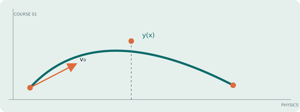
ANCHOR EQUATION
Fountain trajectory
In symbols: y(x) = x tanθ − gx²/(2v₀²cos²θ)
The anchor model for extracting a jet angle and launch speed from a fountain arc.
A fountain arc is an inverse problem
Video of a water jet gives positions; the launch speed and angle are hidden causes. The projectile model predicts a family of arcs, so measuring an arc means estimating parameters and testing whether the residuals look random.
Fit the trajectory, then recover launch data
Use y = Ax − Bx², where A = tanθ and B = g/(2v₀² cos²θ). A quadratic fit supplies A and B. Then θ = arctan A. Since cos²θ = 1/(1 + A²), rearrange B = g(1 + A²)/(2v₀²) to obtain v₀ = √[g(1 + A²)/(2B)]. Each step isolates a physical parameter from the fitted geometry.
If a calibrated video gives y = 0.84x − 0.19x² with x and y in metres, θ = arctan(0.84) = 40.0°. Then v₀ = √[9.81(1 + 0.84²)/(0.38)] = 5.70 m/s. The predicted range at y = 0 is A/B = 4.42 m.
Residuals diagnose the missing physics
Wind and drag usually make the descending branch fall below the ideal parabola. A moving camera can create systematic error in both axes. Fit only a visually selected arc without claiming more precision than the calibration supports.
Work it: Measure five x,y points from a fountain video, fit a quadratic, and calculate θ, v₀, and range. Plot residuals and decide whether the ideal projectile model is defensible.